Present Value Calculation Using Excel
In economics, determining the present value of an income stream is always important because it can help tell the future value of loans, funds, bonds, mortgages, and the like. This is because Present Value Calculation is not as complicated as it sounds. With the help of Excel, it can be easily calculated.
Present Value Calculation Using Excel
Let’s say you have $2,000 in your account after three years. This account pays an interest of 3% annually. How much money do you need to have initially, as an investment, so that you will have that $1,000 by the end of three years.
You can create a present value calculator using Excel by following the steps below:
1. This scenario can be figured out so much easier when you use the Excel spreadsheet as a table to display and track the different variables and time frames for your calculation.
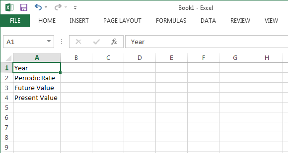
2. Label the cells in Column A as follows: A1 = Years, A2 = Periodic Rate; A3 = Future Value; A4 = Present Value. The table should look like the image below:
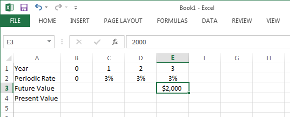
3. Then, in Column B, label the cells in each row as follows: B1 to E1 = Years 0 to 3; B3 to E2 = 3%; E3 = $2,000. Take note that there is no interest earned at time 0, so you put 0 for the periodic rate at Year 0. The future value is also listed to Year 3, where we want to have $2,000.
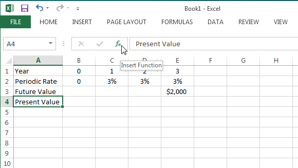
4. Now that the table is complete, calculate the Present Value. Select B4, then click on the Funciton Button (fx) located right above the column labels to populate the Insert Function box.
5. Once the Insert Function box appears, select the “Financial” category from the drop-down list box. Then, choose the PV function from the list that appears. Then, click the “OK” button.
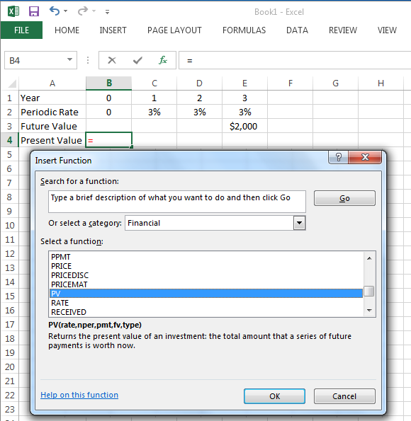
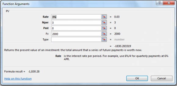
6. Once you click “OK” in the Insert Function box, another box will appear, which is the Function Arguments box. Here, you can type the corresponding values for each given variable. You can use your table for reference. Once you have entered the amounts, the PV calculation will automatically appear at the bottom left-hand corner of the box, which is the “Formula Result.” Then, click “OK” to accept the solution. See the example image below:
7. After accepting the solution, the Formula Result value of your computation will then automatically display in your selected cell, which is B4. This is your PV, or present value. Your table will then look like this:
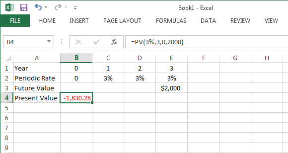
You can see from the example above that the Present Value Calculation appears to be negative because it represents the cash outflow from the investor standpoint.
You can now do the same thing to all your calculations, especially if you are a lender who lends a borrower money with an agreement to have it paid back within a given time frame. Because the lender loses the investment amount of that money, the borrower then has to compensate him in the form of interest. Therefore, the initial amount of the borrowed funds (which is the Present Value) is less than the total amount of the money paid to the lender at the end of the time period.
