How to use VLOOKUP to Find a Value in a Table or Range
So you’ve been organizing your data in Excel. You believe you’ve done a good job so far, but when it comes to looking for a particular piece of information, you spend so much time finding it. If this is you, then you may not have heard about the VLOOOKUP tool in Excel. It has many nifty tools and functions, but the average user probably doesn’t know about them. These tools and functions are most probably left unused. One of these tools is the VLOOKUP, or vertical lookup, tool.
The VLOOKUP tool references vertically aligned tables to quickly and easily find data related to the value that you enter. This is very useful for many applications across many industries using Excel. After all, this Office application is still widely used today. VLOOKUP can be used if you want to find data. For example, if you want to find the price of a product, simply enter it through the VLOOKUP feature and Excel will point you to the data you’re looking for.

How to Use VLOOKUP
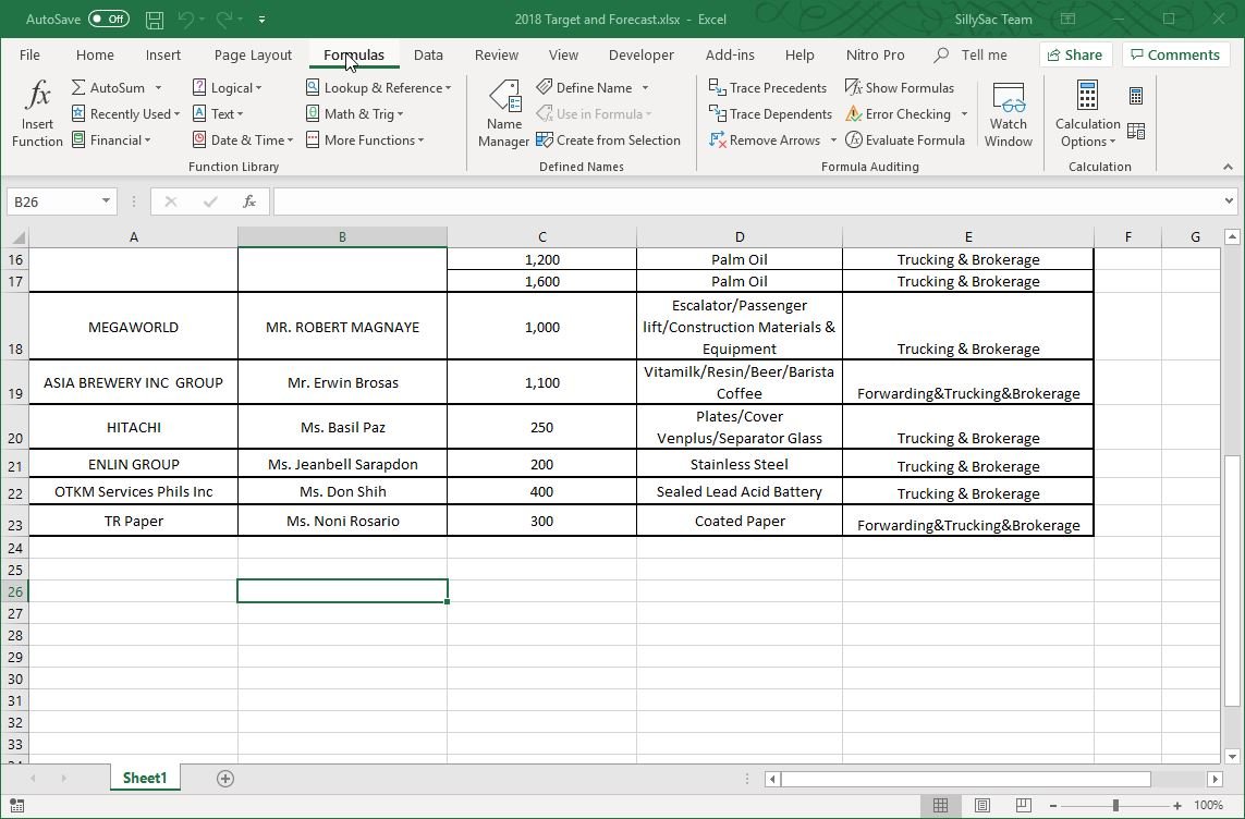
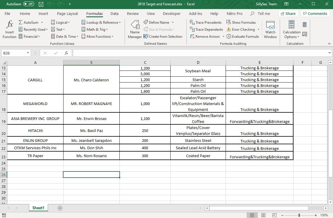
To use VLOOKUP, first click the cell where you want the VLOOKUP formula to appear. This is preferably a blank cell. Then, click “Formulas” in the Ribbon menu. Choose the Lookup & Reference option in the menu under the Formulas tab. This will bring out a drop-down menu, from which you should choose VLOOKUP.

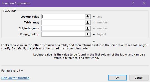
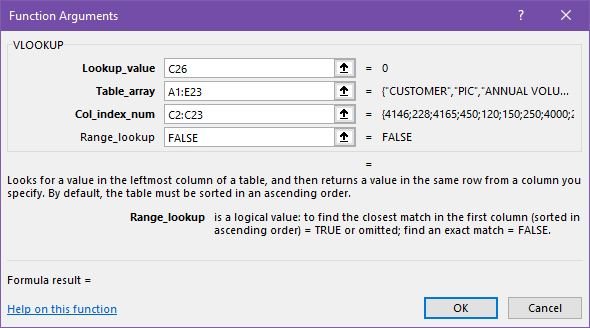
Now, the Function Arguments window will pop out. Here, specify the cell where you will enter the value of the data you’re looking for. In this example, your lookup value is E6. Once you’ve set up the VLOOKUP function properly, you will then see the value you are looking for in C26 whenever you type the data in C25.

Next, specify the data where you want VLOOKUP to search in. This will be in the table_array box in the Function Arguments window. You may choose an entire table or simply select a specific range of the table.

Then, specify the column_index_num, which is the number of the column, instead of the letter designation. You may also specify if you need an exact match. Do this by entering either FALSE (for exact match) or TRUE (for approximate or estimated match) in the range_lookup box. So, if you want an exact match, enter “FALSE”.
Once you’re done, you may click on the OK button. Now, you may go back to your worksheet and table. You can now enter the value of the data you’re searching for, like in the example below.
