How to use IFNA Function in Excel

There is the Excel IF function that creates True or False results. However, if there is an N/A error, there is another function that takes care of that. This is the IFNA function in Excel. In a previous post we showed you how to use the AND function. This time we will show you how to use IFNA function in Excel.

What is the IFNA function in Excel?

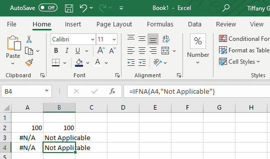
The IFNA function is a logical function that is built-in within Excel along with other functions such as IF, SMALL, or AND functions. The IFNA function allows users to have an alternate value as specified if ever the formula is to have a #N/A error as a return. The IFNA function uses these arguments. First, the Value or the required argument is to have the formula checked for an #N/A error. Then, if there is an error (Value_in_na), the return will have a specified value.

How to use the IFNA function in Excel

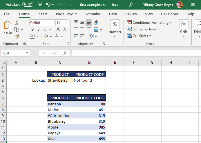
Let’s take a look at this example. Here’s a practical example that is often used in many real-world scenarios. In this  example, the IFNA function is used alongside the VLOOKUP function to create a product search feature in the worksheet. The IFNA function will look for the product “Strawberry” and if the product is not in the list, the IFNA function will work to produce a “Not found” result. This is in replacement to the standard #N/A error value.

The IFNA function in Excel is an excellent way to identify errors in your Excel formulas. Since this trap and handle error function is a Logical function which is used by many Excel enthusiasts in their worksheets. You can also look at other Excel functions and learn about their usage from our guides about Excel functions and formulas. To download various free Excel templates for increasing productivity, see our recommended Excel Productivity Templates.